Contents
- MEEG time-by-time transfer classification
- reduce the number of time points
- Set up chunks
- time-by-time generalization on magneto- and gradio-meters separately
- time-by-time generalization using a searchlight with correlation measure
- Show correlation time-by-time generalization searchlight results
- show citation information
MEEG time-by-time transfer classification
This example shows MVPA generalization across time. The input is a time-locked dataset (chan x time), the output is either:
- (train_time x test_time) indicating for each combination of time points in the training and test set how similar the patterns are
- (train_time x test_time x chan), which uses a searchlight and indicates for each combination of time points in the training and test set how similar the patterns are in the neighborhood of each channel.
Results can be visualized in FieldTrip.
The input dataset involved a paradigm with electrical median nerve stimulation for durations of 2s at 20Hz.
The code presented here can be adapted for other MEEG analyses, but there are a few potential caveats:
- assignment of targets (labels of conditions) is based here on stimulation periods versus pre-stimulation periods. In typical analyses the targets should be based on different trial conditions, for example as set a FieldTrip .trialinfo field.
- the time window used for analyses is rather small. This means that in particular for time-freq analysis a lot of data is missing, especially for early and late timepoints in the lower frequency bands. For typical analyses it may be preferred to use a wider time window.
- the current examples do not perform baseline corrections or signal normalizations, which may reduce discriminatory power.
Note: running this code requires FieldTrip.
- For CoSMoMVPA's copyright information and license terms, #
- see the COPYING file distributed with CoSMoMVPA. #
% set configuration
config = cosmo_config();
data_path = fullfile(config.tutorial_data_path, 'meg_20hz');

% show dataset information
readme_fn = fullfile(data_path, 'README');
cosmo_type(readme_fn);

% reset citation list
cosmo_check_external('-tic');

% load data
data_fn = fullfile(data_path, 'subj102_B01_20Hz_timelock.mat');
data_tl = load(data_fn);

% convert to cosmomvpa struct
ds_tl = cosmo_meeg_dataset(data_tl);

% set the target (trial condition)
ds_tl.sa.targets = ds_tl.sa.trialinfo(:, 1); % 1=pre, 2=peri/post

% set the chunks (independent measurements)
% in this dataset, the first half of the samples (in order)
% are the post-trials;
% the second half the pre-trials
ds_tl.sa.chunks = [(1:145) (1:145)]';

% in addition give a label to each trial
index2label = {'pre', 'post'}; % 1=pre, 2=peri/post
ds_tl.sa.labels = cellfun(@(x)index2label(x), num2cell(ds_tl.sa.targets));

% just to check everything is ok
cosmo_check_dataset(ds_tl);
Summary
-------
MEG data in raw, time-locked and time-frequency formats.

Contents
--------
- subj102_B01_20Hz.fif            raw MEG recording
- preproc.m                       Matlab preprocessing script (based on
                                  FieldTrip)
- subj102_B01_20Hz_timefreq.mat   Time-locked data (generated by preproc.m)
- subj102_B01_20Hz_timelock.mat   Time-frequency data  (generated by preproc.m)
- LICENSE                         License file
- README                          This file

Methods
-------
The dataset involved a paradigm with electrical median nerve stimulation with a
human participant for durations of 2s at 20Hz. Data was acquired at 1khz using
a neuromag306 system.
Trial info in the .mat files: 1=pre-stimulus, 2=peri/post-stimulus

License
-------
The contents are made available by Nathan Weisz <nathanweisz |at| me.com> and
Gianpaolo Demarchi <gianpaolo.demarchi |at| unitn.it> under the Creative
Commons CC0 1.0 Universal Public Domain Dedication ("CC0"). See the LICENSE
file for details, or visit
http://creativecommons.org/publicdomain/zero/1.0/deed.en.

Acknowledgements
----------------
Thanks to Nathan Weisz and Gianpaolo Demarchi for providing this dataset, and
an anonymous participant for volunteering during the recordings.

Contact
-------
Nikolaas N. Oosterhof <nikolaas.oosterhof |at| unitn.it>
reduce the number of time points
to allow this example to run relatively fast, only use the 'even' timepoints and only use timepoints between 0 and 300 ms relative to stimulus onset. for a publication-quality analysis this step could be omitted.
msk = cosmo_dim_match(ds_tl, 'time', @(x) 0 < x & x < .3) & ...
                        mod(ds_tl.fa.time, 2) == 0;
ds = cosmo_slice(ds_tl, msk, 2);
ds = cosmo_dim_prune(ds);
Set up chunks
use half of the data for training and half for testing. Here both chunks come from the same session, but it is also possible to use different sessions for training and testing.
For example, the train data can contain responses to auditory stimuli with the words 'face' and 'house', while the test session measures responses to visual stimuli. In that case the chunks should be assigned 'manually' (without cosmo_chunkize)
nchunks = 2; % two chunks are required for this analysis
ds.sa.chunks = cosmo_chunkize(ds, nchunks);
time-by-time generalization on magneto- and gradio-meters separately
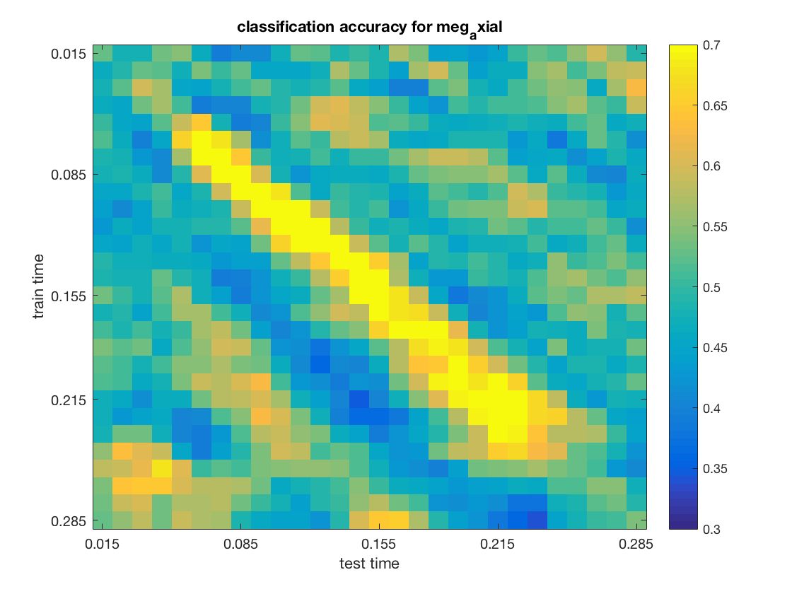
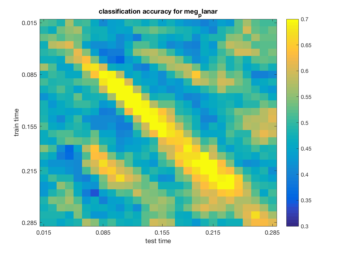
compute and plot accuracies for magnetometers and gradiometers separately
chan_types = {'meg_axial', 'meg_planar'};
nchan_types = numel(chan_types);

% set arguments for the cosmo_dim_generalization_measure
measure_args = struct();

% the cosmo_dim_generalization_measure requires that another
% measure (here: the crossvalidation measure) is specified. The
% specified measure is applied for each combination of time points
measure_args.measure = @cosmo_crossvalidation_measure;

% When used ordinary, the cosmo_crossvalidation_measure itself
% requires two arguments:
% - classifier (here: LDA)
% - partitions
% However, because the cosmo_dim_generalization_measure defines
% the partitions itself, they are not set here.
measure_args.classifier = @cosmo_classify_lda;

% define the dimension over which generalization takes place
measure_args.dimension = 'time';

% define the radius for the time dimension. Here not just a single
% time-point is used, but also the time-point before it and the time-point
% after it.
measure_args.radius = 1;

% try both channel types (axial and planar)
for k = 1:nchan_types
    use_chan_type = chan_types{k};

    % get layout for mag or planar labels, and select only those channels
    ds_chan_types = cosmo_meeg_chantype(ds);
    ds_chan_idxs = find(cosmo_match(ds_chan_types, use_chan_type));
    feature_msk = cosmo_match(ds.fa.chan, ds_chan_idxs);
    ds_sel = cosmo_slice(ds, feature_msk, 2);

    % make 'time' a sample dimension
    % (this necessary for cosmo_dim_generalization_measure)
    ds_time = cosmo_dim_transpose(ds_sel, 'time', 1);

    fprintf('The input for channel type %s is:\n', use_chan_type);
    cosmo_disp(ds_time);

    % run transfer across time with the searchlight neighborhood
    % cdt_ds=cosmo_cartesian_dim_transfer(ds_time,'time',measure,...
    %                        'args',measure_args);
    cdt_ds = cosmo_dim_generalization_measure(ds_time, measure_args);

    fprintf('The output is:\n');
    cosmo_disp(cdt_ds);

    % unflatten the data to get train_time x test_time matrix
    [data, labels, values] = cosmo_unflatten(cdt_ds, 1);

    % show the results
    figure();
    imagesc(data, [.3 .7]);
    title(sprintf('classification accuracy for %s', use_chan_type));
    colorbar();
    nticks = 5;

    ytick = round(linspace(1, numel(values{1}), nticks));
    ylabel(strrep(labels{1}, '_', ' '));
    set(gca, 'Ytick', ytick, 'YTickLabel', values{1}(ytick));

    xtick = round(linspace(1, numel(values{2}), nticks));
    xlabel(strrep(labels{2}, '_', ' '));
    set(gca, 'Xtick', xtick, 'XTickLabel', values{2}(xtick));

    colorbar();
end
The input for channel type meg_axial is:
.samples
  [  2.94e-13  1.53e-13  2.36e-13  ...   1.19e-13  7.72e-14 -2.62e-14
     3.24e-13  1.97e-13   2.4e-13  ...  -1.75e-13 -2.26e-13 -1.94e-13
    -1.33e-13 -1.83e-13 -1.25e-13  ...  -1.62e-13 -7.59e-14  4.23e-14
        :         :         :               :         :         :
    -2.45e-13 -2.22e-13 -2.82e-13  ...   8.02e-14  1.61e-13  1.41e-13
     1.15e-14 -3.43e-14 -1.05e-13  ...  -1.96e-14 -4.12e-14  5.86e-15
      1.9e-13  1.78e-13  2.86e-13  ...  -3.17e-13 -2.42e-13 -3.42e-13 ]@8700x101
.sa
  .chunks
    [ 1
      2
      1
      :
      1
      2
      1 ]@8700x1
  .labels
    { 'post'
      'post'
      'post'
        :
      'pre'
      'pre'
      'pre'  }@8700x1
  .targets
    [ 2
      2
      2
      :
      1
      1
      1 ]@8700x1
  .time
    [  1
       1
       1
       :
      30
      30
      30 ]@8700x1
  .trialinfo
    [ 2         1
      2         2
      2         3
      :        :
      1       148
      1       149
      1       150 ]@8700x2
.fa
  .chan
    [ 3         6         9  ...  297       300       303 ]@1x101
  .transpose_ids
    [ 1         2         3  ...  99       100       101 ]@1x101
.a
  .fdim
    .labels
      { 'chan' }
    .values
      { { 'MEG0113'  'MEG0112'  'MEG0111' ... 'MEG2642'  'MEG2643'  'MEG2641'   }@1x303 }
  .meeg
    .samples_field
      'trial'
  .sdim
    .labels
      { 'time' }
    .values
      { [ 0.005
          0.015
          0.025
            :
          0.275
          0.285
          0.295 ]@30x1 }
+00:00:01 [####################] -00:00:00
The output is:
.samples
  [ 0.528
    0.479
    0.479
      :
      0.5
    0.507
    0.542 ]@784x1
.sa
  .labels
    { 'accuracy'
      'accuracy'
      'accuracy'
          :
      'accuracy'
      'accuracy'
      'accuracy' }@784x1
  .test_time
    [  1
       2
       3
       :
      26
      27
      28 ]@784x1
  .train_time
    [  1
       1
       1
       :
      28
      28
      28 ]@784x1
.a
  .sdim
    .labels
      { 'train_time'  'test_time' }
    .values
      { [ 0.015         [ 0.015
          0.025           0.025
          0.035           0.035
            :               :
          0.265           0.265
          0.275           0.275
          0.285 ]@28x1    0.285 ]@28x1 }
The input for channel type meg_planar is:
.samples
  [  1.88e-12     9e-12  6.47e-12  ...  -4.35e-12 -4.44e-12  5.89e-12
        4e-12  8.53e-12   8.8e-12  ...  -9.94e-12  3.98e-12  8.68e-13
    -7.51e-12  5.93e-12 -1.66e-12  ...  -2.57e-12 -5.51e-12 -4.38e-14
        :         :         :               :         :         :
      3.8e-12 -1.76e-12 -4.97e-12  ...  -3.09e-12     1e-12  4.24e-13
    -3.85e-12 -2.32e-12  4.86e-12  ...   1.19e-12  3.11e-12  1.18e-12
    -5.57e-12  2.88e-12 -4.12e-13  ...   4.88e-13  5.98e-13 -2.75e-12 ]@8700x202
.sa
  .chunks
    [ 1
      2
      1
      :
      1
      2
      1 ]@8700x1
  .labels
    { 'post'
      'post'
      'post'
        :
      'pre'
      'pre'
      'pre'  }@8700x1
  .targets
    [ 2
      2
      2
      :
      1
      1
      1 ]@8700x1
  .time
    [  1
       1
       1
       :
      30
      30
      30 ]@8700x1
  .trialinfo
    [ 2         1
      2         2
      2         3
      :        :
      1       148
      1       149
      1       150 ]@8700x2
.fa
  .chan
    [ 1         2         4  ...  299       301       302 ]@1x202
  .transpose_ids
    [ 1         2         3  ...  200       201       202 ]@1x202
.a
  .fdim
    .labels
      { 'chan' }
    .values
      { { 'MEG0113'  'MEG0112'  'MEG0111' ... 'MEG2642'  'MEG2643'  'MEG2641'   }@1x303 }
  .meeg
    .samples_field
      'trial'
  .sdim
    .labels
      { 'time' }
    .values
      { [ 0.005
          0.015
          0.025
            :
          0.275
          0.285
          0.295 ]@30x1 }
+00:00:01 [####################] -00:00:00
The output is:
.samples
  [ 0.514
    0.507
    0.486
      :
    0.625
    0.625
    0.611 ]@784x1
.sa
  .labels
    { 'accuracy'
      'accuracy'
      'accuracy'
          :
      'accuracy'
      'accuracy'
      'accuracy' }@784x1
  .test_time
    [  1
       2
       3
       :
      26
      27
      28 ]@784x1
  .train_time
    [  1
       1
       1
       :
      28
      28
      28 ]@784x1
.a
  .sdim
    .labels
      { 'train_time'  'test_time' }
    .values
      { [ 0.015         [ 0.015
          0.025           0.025
          0.035           0.035
            :               :
          0.265           0.265
          0.275           0.275
          0.285 ]@28x1    0.285 ]@28x1 }
time-by-time generalization using a searchlight with correlation measure
how many channel locations in each searchlight
nchannel_locations_searchlight = 10;

% make 'time' a sample dimension (necessary for cartesian_dim_transfer)
ds_time = cosmo_dim_transpose(ds_sel, 'time', 1);

% use planar channels as input; output is
% like combine-planar
use_chan_type = 'meg_combined_from_planar';

% define searchlight neighborhood
nbrhood = cosmo_meeg_chan_neighborhood(ds_time, ...
                                       'count', nchannel_locations_searchlight, ...
                                       'chantype', use_chan_type);

fprintf('The input is:\n');
cosmo_disp(ds_time);

fprintf('The neighborhood is:\n');
cosmo_disp(nbrhood);

% set the measure to be the dim generalization measure
measure = @cosmo_dim_generalization_measure;

% define the arguments for the measure. One of them is called 'measure',
% because that measure is applied to combinations of samples in the
% train and test set
measure_args = struct();
measure_args.measure = @cosmo_correlation_measure;
measure_args.radius = 1;
measure_args.dimension = 'time';

% run transfer across time with the searchlight neighborhood
cdt_ds = cosmo_searchlight(ds_time, nbrhood, measure, measure_args);

fprintf('The output is:\n');
cosmo_disp(cdt_ds);

% move {train,test}_time from being sample dimensions to feature
% dimensions, so they can be mapped to a fieldtrip struct
cdt_tf_ds = cosmo_dim_transpose(cdt_ds, {'train_time', 'test_time'}, 2);

fprintf('The output after transposing is:\n');
cosmo_disp(cdt_ds);

% trick fieldtrip into thinking this is a time-freq-chan dataset, by
% renaming train_time and test_time to freq and time, respectively
cdt_tf_ds = cosmo_dim_rename(cdt_tf_ds, 'train_time', 'freq');
cdt_tf_ds = cosmo_dim_rename(cdt_tf_ds, 'test_time', 'time');
The input is:
.samples
  [  1.88e-12     9e-12  6.47e-12  ...  -4.35e-12 -4.44e-12  5.89e-12
        4e-12  8.53e-12   8.8e-12  ...  -9.94e-12  3.98e-12  8.68e-13
    -7.51e-12  5.93e-12 -1.66e-12  ...  -2.57e-12 -5.51e-12 -4.38e-14
        :         :         :               :         :         :
      3.8e-12 -1.76e-12 -4.97e-12  ...  -3.09e-12     1e-12  4.24e-13
    -3.85e-12 -2.32e-12  4.86e-12  ...   1.19e-12  3.11e-12  1.18e-12
    -5.57e-12  2.88e-12 -4.12e-13  ...   4.88e-13  5.98e-13 -2.75e-12 ]@8700x202
.sa
  .chunks
    [ 1
      2
      1
      :
      1
      2
      1 ]@8700x1
  .labels
    { 'post'
      'post'
      'post'
        :
      'pre'
      'pre'
      'pre'  }@8700x1
  .targets
    [ 2
      2
      2
      :
      1
      1
      1 ]@8700x1
  .time
    [  1
       1
       1
       :
      30
      30
      30 ]@8700x1
  .trialinfo
    [ 2         1
      2         2
      2         3
      :        :
      1       148
      1       149
      1       150 ]@8700x2
.fa
  .chan
    [ 1         2         4  ...  299       301       302 ]@1x202
  .transpose_ids
    [ 1         2         3  ...  200       201       202 ]@1x202
.a
  .fdim
    .labels
      { 'chan' }
    .values
      { { 'MEG0113'  'MEG0112'  'MEG0111' ... 'MEG2642'  'MEG2643'  'MEG2641'   }@1x303 }
  .meeg
    .samples_field
      'trial'
  .sdim
    .labels
      { 'time' }
    .values
      { [ 0.005
          0.015
          0.025
            :
          0.275
          0.285
          0.295 ]@30x1 }
The neighborhood is:
.neighbors
  { [ 1         2         3  ...  24       109       110 ]@1x20
    [ 1         2         3  ...  24        39        40 ]@1x20
    [ 1         2         3  ...  24       109       110 ]@1x20
                                  :
    [ 97        98       105  ...  200       201       202 ]@1x19
    [ 174       175       181  ...  200       201       202 ]@1x20
    [ 97        98       180  ...  200       201       202 ]@1x19  }@102x1
.fa
  .chan
    [ 1         2         3  ...  100       101       102 ]@1x10²
.a
  .fdim
    .labels
      { 'chan' }
    .values
      { { 'MEG0112+0113'  'MEG0122+0123'  'MEG0132+0133' ... 'MEG2622+2623'  'MEG2632+2633'  'MEG2642+2643'   }@1x10² }
  .meeg
    .samples_field
      'trial'
.origin
  .fa
    .chan
      [ 1         2         4  ...  299       301       302 ]@1x202
    .transpose_ids
      [ 1         2         3  ...  200       201       202 ]@1x202
  .a
    .fdim
      .labels
        { 'chan' }
      .values
        { { <char>@1x7  <char>@1x7  <char>@1x7 ... <char>@1x7  <char>@1x7  <char>@1x7   }@1x303 }
    .meeg
      .samples_field
        'trial'
    .sdim
      .labels
        { 'time' }
      .values
        { [ 0.005
            0.015
            0.025
              :
            0.275
            0.285
            0.295 ]@30x1 }
+00:00:42 [####################] -00:00:00
The output is:
.a
  .fdim
    .labels
      { 'chan' }
    .values
      { { 'MEG0112+0113'  'MEG0122+0123'  'MEG0132+0133' ... 'MEG2622+2623'  'MEG2632+2633'  'MEG2642+2643'   }@1x10² }
  .meeg
    .samples_field
      'trial'
  .sdim
    .labels
      { 'train_time'  'test_time' }
    .values
      { [ 0.015         [ 0.015
          0.025           0.025
          0.035           0.035
            :               :
          0.265           0.265
          0.275           0.275
          0.285 ]@28x1    0.285 ]@28x1 }
.fa
  .chan
    [ 1         2         3  ...  100       101       102 ]@1x10²
  .center_ids
    [ 1         2         3  ...  100       101       102 ]@1x10²
.samples
  [ -0.00468    0.0748   -0.0547  ...  0.331      0.28     0.232
      -0.125    0.0217    -0.151  ...  0.336      0.22     0.264
      -0.178   -0.0212    -0.177  ...  0.305      0.22     0.285
        :         :         :            :         :         :
     -0.0953  -0.00198     0.176  ...  0.134     0.413     0.329
     -0.0145     0.177     0.194  ...  0.232     0.468     0.431
       0.116     0.326     0.278  ...   0.25     0.401     0.414 ]@784x102
.sa
  .labels
    { 'corr'
      'corr'
      'corr'
        :
      'corr'
      'corr'
      'corr' }@784x1
  .test_time
    [  1
       2
       3
       :
      26
      27
      28 ]@784x1
  .train_time
    [  1
       1
       1
       :
      28
      28
      28 ]@784x1
The output after transposing is:
.a
  .fdim
    .labels
      { 'chan' }
    .values
      { { 'MEG0112+0113'  'MEG0122+0123'  'MEG0132+0133' ... 'MEG2622+2623'  'MEG2632+2633'  'MEG2642+2643'   }@1x10² }
  .meeg
    .samples_field
      'trial'
  .sdim
    .labels
      { 'train_time'  'test_time' }
    .values
      { [ 0.015         [ 0.015
          0.025           0.025
          0.035           0.035
            :               :
          0.265           0.265
          0.275           0.275
          0.285 ]@28x1    0.285 ]@28x1 }
.fa
  .chan
    [ 1         2         3  ...  100       101       102 ]@1x10²
  .center_ids
    [ 1         2         3  ...  100       101       102 ]@1x10²
.samples
  [ -0.00468    0.0748   -0.0547  ...  0.331      0.28     0.232
      -0.125    0.0217    -0.151  ...  0.336      0.22     0.264
      -0.178   -0.0212    -0.177  ...  0.305      0.22     0.285
        :         :         :            :         :         :
     -0.0953  -0.00198     0.176  ...  0.134     0.413     0.329
     -0.0145     0.177     0.194  ...  0.232     0.468     0.431
       0.116     0.326     0.278  ...   0.25     0.401     0.414 ]@784x102
.sa
  .labels
    { 'corr'
      'corr'
      'corr'
        :
      'corr'
      'corr'
      'corr' }@784x1
  .test_time
    [  1
       2
       3
       :
      26
      27
      28 ]@784x1
  .train_time
    [  1
       1
       1
       :
      28
      28
      28 ]@784x1
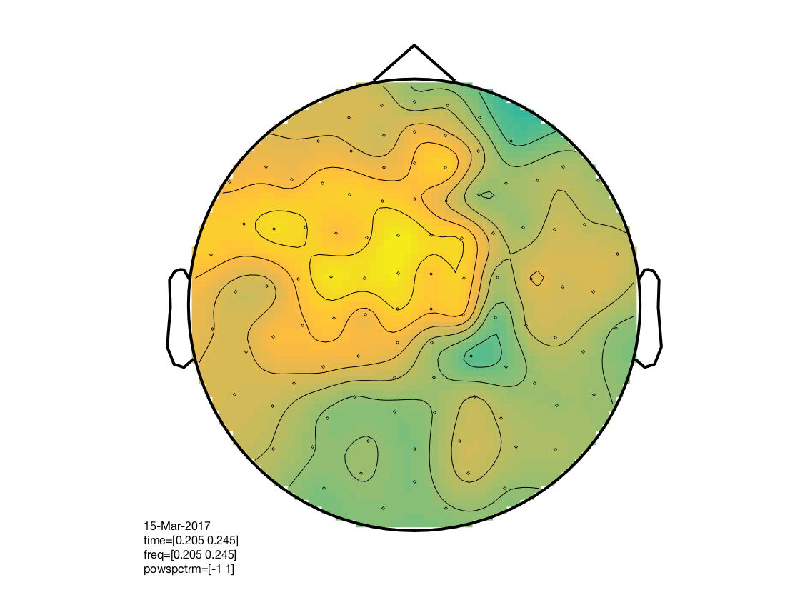
Show correlation time-by-time generalization searchlight results
% determine layout
layout = cosmo_meeg_find_layout(cdt_tf_ds);

% convert to fieldtrip format
ft = cosmo_map2meeg(cdt_tf_ds);

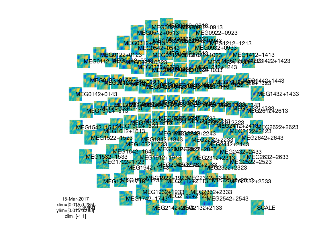
% show train_time x test_time x chan figure
%
% * train_time is on the vertical ('freq') axis
% * test_time on the horizontal ('time') axis)
figure();
cfg = [];
cfg.interactive = 'yes';
cfg.showlabels = 'yes';
cfg.zlim = [-1 1];
cfg.layout       = layout;
ft_multiplotTFR(cfg, ft);

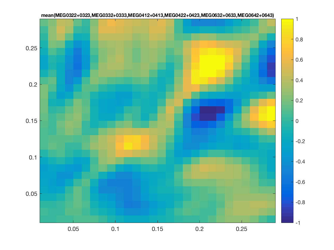
% show train_time x test_time figure for selected channels
figure();
cfg = [];
cfg.interactive = 'yes';
cfg.showlabels = 'yes';
cfg.zlim = [-1 1];
cfg.layout       = layout;
cfg.channel = {'MEG0322+0323', 'MEG0332+0333', 'MEG0412+0413', ...
               'MEG0422+0423', 'MEG0632+0633', 'MEG0642+0643'};

ft_singleplotTFR(cfg, ft);

% show channel topology for timewindow over train_time x test_time
figure();
cfg = [];
cfg.interactive = 'yes';
cfg.xlim = [.2 .25];
cfg.ylim = [.2 .25];
cfg.zlim = [-1 1];
cfg.layout       = layout;
ft_topoplotTFR(cfg, ft);
the call to "ft_selectdata" took 0 seconds and required the additional allocation of an estimated NaN MB
the call to "ft_prepare_layout" took 0 seconds and required the additional allocation of an estimated NaN MB
the call to "ft_multiplotTFR" took 0 seconds and required the additional allocation of an estimated NaN MB
the call to "ft_selectdata" took 0 seconds and required the additional allocation of an estimated NaN MB
the call to "ft_singleplotTFR" took 0 seconds and required the additional allocation of an estimated NaN MB
the call to "ft_prepare_layout" took 0 seconds and required the additional allocation of an estimated NaN MB
the call to "ft_selectdata" took 0 seconds and required the additional allocation of an estimated NaN MB
the call to "ft_topoplotTFR" took 0 seconds and required the additional allocation of an estimated NaN MB
show citation information
cosmo_check_external('-cite');
If you use CoSMoMVPA and/or some other toolboxes for a publication, please cite:

R. Oostenveld, P. Fries, E. Maris, J.-M. Schoffelen (2011). FieldTrip: Open Source Software for Advanced Analysis of MEG, EEG, and Invasive Electrophysiological Data, Computational Intelligence and Neuroscience, vol. 2011, Article ID 156869, 9 pages.doi:10.1155/2011/156869. FieldTrip toolbox available online from http://fieldtrip.fcdonders.nl

N. N. Oosterhof, A. C. Connolly, J. V. Haxby (2016). CoSMoMVPA: multi-modal multivariate pattern analysis of neuroimaging data in Matlab / GNU Octave. Frontiers in Neuroinformatics, doi:10.3389/fninf.2016.00027.. CoSMoMVPA toolbox available online from http://cosmomvpa.org

The Mathworks, Natick, MA, United States. Matlab 24.1.0.2537033 (R2024a) (February 21, 2024). available online from http://www.mathworks.com