Contents
- Anatomical dataset basics
- Show the dataset contents using cosmo_disp. Where can you see the
- There are a lot of zero values in the dataset. Find all non-zero values
- Using cosmo_plot_slices, show a sagittal view of the dataset
- ds.fa.i contains, for each feature (voxel), an index for the
- Advanced exercise: set all voxels around a center voxel at
Anatomical dataset basics
In this example, load a brain as a CoSMoMVPA dataset and visualize it in matlab
- For CoSMoMVPA's copyright information and license terms, #
- see the COPYING file distributed with CoSMoMVPA. #
% Set the path.
config = cosmo_config();
data_path = fullfile(config.tutorial_data_path, 'ak6', 's01');

% Set filename
fn = fullfile(data_path, 'brain.nii');

% Load with cosmo_fmri_dataset and assign to a variable 'ds'
% >@@>
ds = cosmo_fmri_dataset(fn);
% <@@<
Show the dataset contents using cosmo_disp. Where can you see the
number of voxels in the three spatial dimensions? >@@>
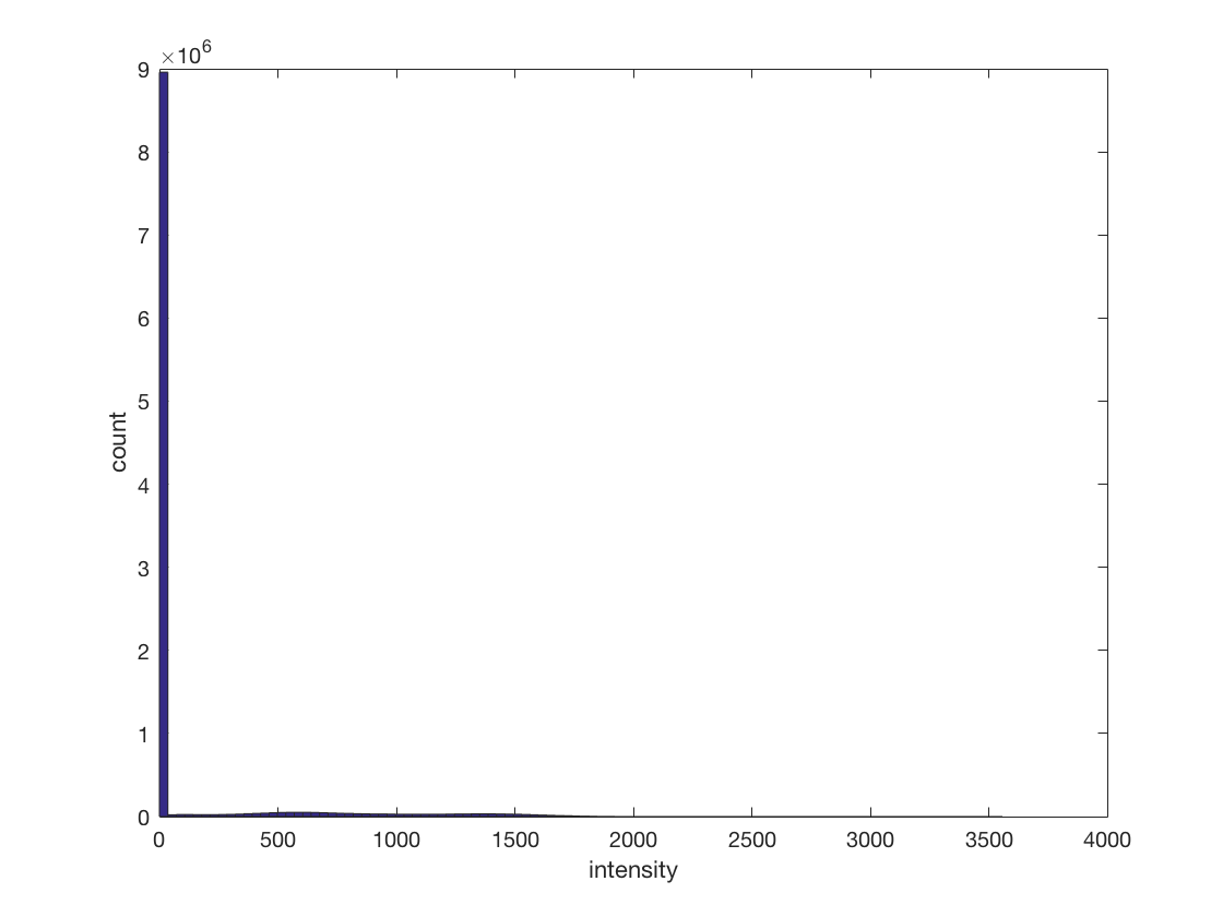
cosmo_disp(ds);

% the number of voxels in the spatial dimensions are present in
% ds.a.vol.dim, and are also indicated by the sizes of ds.a.fdim.values
% <@@<

% Show a histogram of all values in the dataset. For bonus points add axis
% labels.
% Hint: all data is present in ds.samples
% >@@>
hist(ds.samples, 100);
xlabel('intensity');
ylabel('count');
% <@@<
.a
  .vol
    .mat
      [      0         0         1     -84.9
        -0.938         0         0       124
             0     0.938         0     -65.8
             0         0         0         1 ]
    .xform
      'scanner_anat'
    .dim
      [ 256       256       160 ]
  .fdim
    .labels
      { 'i'
        'j'
        'k' }
    .values
      { [ 1         2         3  ...  254       255       256 ]@1x256
        [ 1         2         3  ...  254       255       256 ]@1x256
        [ 1         2         3  ...  158       159       160 ]@1x160 }
.sa
  struct (empty)
.samples
  [ 0         0         0  ...  0         0         0 ]@1x10485760
.fa
  .i
    [ 1         2         3  ...  254       255       256 ]@1x10485760
  .j
    [ 1         1         1  ...  256       256       256 ]@1x10485760
  .k
    [ 1         1         1  ...  160       160       160 ]@1x10485760
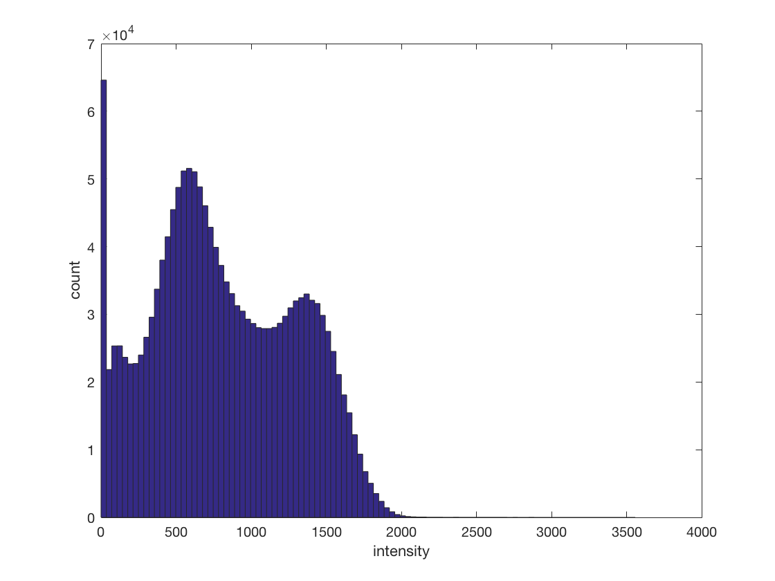
There are a lot of zero values in the dataset. Find all non-zero values
in ds.samples, and plot a histogram of those. What do the two bumps represent? >@@>
nonzero_mask = ds.samples ~= 0;
nonzero_samples = ds.samples(ds.samples ~= 0);
hist(nonzero_samples, 100);
xlabel('intensity');
ylabel('count');
% <@@<
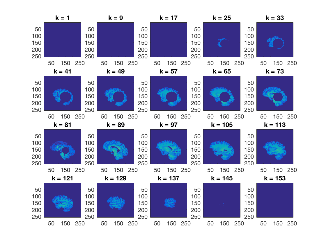
Using cosmo_plot_slices, show a sagittal view of the dataset
>@@>
cosmo_plot_slices(ds);
% <@@<

% Make a copy of the dataset
ds_copy = ds;

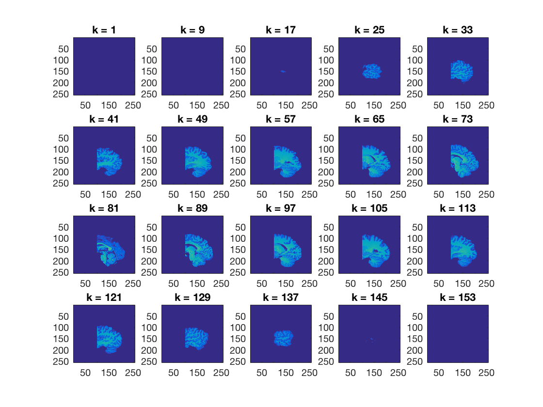
ds.fa.i contains, for each feature (voxel), an index for the
anterior-posterior position of that voxel. Set all voxels that have a value of less than 100 for ds.fa.i to zero, and plot the results >@@>
ds_copy.samples(ds.fa.i < 100) = 0;
cosmo_plot_slices(ds_copy);
% <@@<

% Store the results in a nifti file for visualization using cosmo_map2fmri
output_path = config.output_data_path;
fn_out = fullfile(output_path, 'anatomical_dataset_posterior.nii');
% >@@>
cosmo_map2fmri(ds_copy, fn_out);
% <@@<
Advanced exercise: set all voxels around a center voxel at
i=150,j=100,k=50 within a 40-voxel radius to zero, and display the result
center_ijk = [150; 100; 50];
radius = 40;
% >@@>
ds_copy2 = ds;
all_ijk = [ds_copy2.fa.i; ...
           ds_copy2.fa.j; ...
           ds_copy2.fa.k];

% compute difference dimension-wise
delta = bsxfun(@minus, center_ijk, all_ijk);

% Pythogoras
squared_distance_from_center = sum(delta.^2, 1);

% define mask
mask = squared_distance_from_center <= radius^2;

% set voxels to zero
ds_copy2.samples(:, mask) = 0;

% show result
cosmo_plot_slices(ds_copy2);
% <@@<