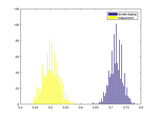
Double dipping

% Warning: this exercise shows the *bad* practice of double dipping
% (also known as circular analysis). You must never, ever use
% results double dipping to interpret results for a real analysis that you
% would publish.

nfeatures = 100;
nsamples_per_class = 200;
nclasses = 2;
niter = 1000;

% compute number of samples
nsamples = nclasses * nsamples_per_class;

% set targets
targets = repmat((1:nclasses)', nsamples_per_class, 1);

% allocate space for output
accuracies = zeros(niter, 2);

for iter = 1:niter
    % generate random gaussian train data of size nsamples x nfeatures
    % assign the result to a variable 'train_data'
    % >@@>
    train_data = randn(nsamples, nfeatures);
    % <@@<

    % for the double dipping test data, assign 'double_dipping_test_data'
    % to be the same as the training data.
    %
    % *** WARNING ***
    % For real data analyses (that you would publish in a paper) you
    % must never do double dipping analysis - its results are invalid
    % ****************
    % >@@>
    double_dipping_test_data = train_data;
    % <@@<

    % for the independent data, generate random gaussian data (of the
    % same size as train_data) and assign to a variable
    % 'independent_test_data'
    % >@@>
    independent_test_data = randn(nsamples, nfeatures);
    % <@@<

    % compute class labels predictions for both test sets using
    % cosmo_classify_lda. Store the predictions in
    % 'double_dipping_pred' and 'independent_pred', respectively
    % >@@>
    double_dipping_pred = cosmo_classify_lda(train_data, targets, ...
                                             double_dipping_test_data);
    independent_pred = cosmo_classify_lda(train_data, targets, ...
                                          independent_test_data);
    % <@@<

    % compute classification accuracies
    double_dipping_acc = mean(double_dipping_pred == targets);
    independent_acc = mean(independent_pred == targets);

    % store accuracies in the iter-th row of the 'accuracies' matrix
    % >@@>
    accuracies(iter, :) = [double_dipping_acc, independent_acc];
    % <@@<
end

% show histogram
hist(accuracies, 100);
legend({'double dipping', 'independent'});