RSA Tutorial

Compare DSMs

For CoSMoMVPA's copyright information and license terms, #
see the COPYING file distributed with CoSMoMVPA. #

subjects = {'s01', 's02', 's03', 's04', 's05', 's06', 's07', 's08'};
masks = {'ev_mask.nii', 'vt_mask.nii'};

config = cosmo_config();
study_path = fullfile(config.tutorial_data_path, 'ak6');

In a nested loop over masks then subjects: load each dataset demean it, get DSM, save it in dsms

n_subjects = numel(subjects);
n_masks = numel(masks);

counter = 0;

for m = 1:n_masks
    msk = masks{m};
    for s = 1:length(subjects)
        sub = subjects{s};
        sub_path = fullfile(study_path, sub);

        % load dataset
        ds_fn = fullfile(sub_path, 'glm_T_stats_perrun.nii');
        mask_fn = fullfile(sub_path, msk);
        ds_full = cosmo_fmri_dataset(ds_fn, ...
                                     'mask', mask_fn, ...
                                     'targets', repmat(1:6, 1, 10)');

        % compute average for each unique target
        ds = cosmo_fx(ds_full, @(x)mean(x, 1), 'targets', 1);

        % remove constant features
        ds = cosmo_remove_useless_data(ds);

        % demean
        % Comment this out to see the effects of demeaning vs. not
        ds.samples = bsxfun(@minus, ds.samples, mean(ds.samples, 1));

        % compute the one-minus-correlation value for each pair of
        % targets.
        % (Hint: use cosmo_pdist with the 'correlation' argument)
        % >@@>
        dsm = cosmo_pdist(ds.samples, 'correlation');
        % <@@<

        if counter == 0
            % first dsm, allocate space
            n_pairs = numel(dsm);
            neural_dsms = zeros(n_subjects * n_masks, n_pairs);
        end

        % increase counter and store the dsm as the counter-th row in
        % 'neural_dsms'
        % >@@>
        counter = counter + 1;
        neural_dsms(counter, :) = dsm;
        % <@@<
    end
end

Then add the v1 model and behavioral DSMs

models_path = fullfile(study_path, 'models');
load(fullfile(models_path, 'v1_model.mat'));
load(fullfile(models_path, 'behav_sim.mat'));
% add to dsms (hint: use comso_squareform)
% >@@>
v1_model_sf = cosmo_squareform(v1_model);
behav_model_sf = cosmo_squareform(behav);
% ensure row vector because Matlab and Octave return
% row and column vectors, respectively
dsms = [neural_dsms; v1_model_sf(:)'; behav_model_sf(:)'];
% <@@<

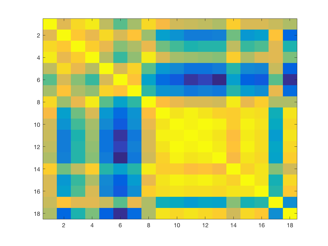
Now visualize the cross-correlation matrix. Remember that 'cosmo_corr' (or the builtin 'corr') calculates correlation coefficients between columns and we want between rows, so the data has to be transposed.

% >@@>
cc = cosmo_corr(dsms');
figure();
imagesc(cc);
% <@@<

Now use the values in the last two rows of the cross correlation matrix to visualize the distributions in correlations between the neural similarities and the v1 model/behavioral ratings. Store the result in a matrix 'cc_models', which should have 8 rows (corresponding to the participants) and 4 columns (corresponding to EV and VT correlated with both models)

Rows 1 to 8: EV neural similarities Rows 9 to 16: VT neural similarities Row 17: EV model Row 18: behavioural similarities

% >@@>
cc_models = [cc(1:8, 17) cc(9:16, 17) cc(1:8, 18) cc(9:16, 18)];
% <@@<
labels = {'v1 model~EV', 'v1 model~VT', 'behav~EV', 'behav~VT'};
figure();
boxplot(cc_models);
set(gca, 'XTick', [1:4], 'XTickLabel', labels);