Multiple comparison correction with Threshold-Free Cluster Enhancement

This example demonstrates cosmo_cluster_neighborhood and cosmo_montecarlo_cluster_stat

Note: this example shows multiple-comparison for a single subject, but the same logic can be applied to a group of subjects to do a group analysis.

Contents

Define data

config = cosmo_config();
data_path = fullfile(config.tutorial_data_path, 'ak6', 's01');

targets = repmat(1:6, 1, 10);
chunks = floor(((1:60) - 1) / 6) + 1;

ds = cosmo_fmri_dataset(fullfile(data_path, 'glm_T_stats_perrun.nii'), ...
                        'mask', fullfile(data_path, 'brain_mask.nii'), ...
                        'targets', targets, 'chunks', chunks);

% There are 10 chunks, for which the data is assumed to be independent.
% Construct a dataset with 10 samples corresponding to each chunk, with
% the average value across all six targets. Each sample is considered to be
% the same condition, namely the effect of the stimulus-versus-baseline
% effect; thus all target values must be set to 1.
%
% Use either:
%   - cosmo_split and cosmo_stack
%   - cosmo_average_samples
%   - (advanced) cosmo_fx
%
% Assign the result to a variable 'ds_stim'
% >@@>
ds_stim = cosmo_fx(ds, @(x)mean(x, 1), {'chunks'});

% % alternative:
%     ds_stim=ds;
%     ds_stim.sa.targets(:)=1;
%     ds_split=cosmo_split(ds_stim,{'chunks'});
%
%     for k=1:numel(ds_split)
%         ds_avg_k=cosmo_slice(ds_split{k},1);
%         ds_avg_k.samples=mean(ds_split{k}.samples,1);
%         ds_split{k}=ds_avg_k;
%     end
%
%     ds_stim=cosmo_stack(ds_split);
%
% <@@<

Define a cluster neighborhood for this dataset and assign the result to

a variable 'cl_nh'. hint: use cosmo_cluster_neighborhood

% >@@>
cl_nh = cosmo_cluster_neighborhood(ds_stim);
% <@@<

% Show a plot with the sorted number of neighbors
% for each voxel

% >@@>
n_neighbors_per_feature = cellfun(@numel, cl_nh.neighbors);
plot(sort(n_neighbors_per_feature));
% <@@<

+00:00:00 [####################] -00:00:00  mean size 25.5

Run cosmo_montecarlo_cluster_stat

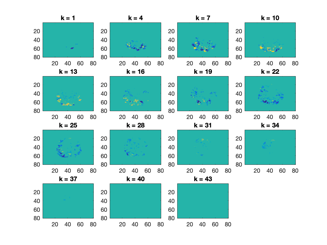
% There is one condition per chunk; all targets are set to 1.
% Thus the subsequent analysis is a one-sample t-test.
% Note: if this was a group analysis, then each sample (row in ds.samples)
% would contain data from one subject; each unique value in .sa.chunks
% would correspond to one subject; and each unique value in .sa.targets
% would correspond to a condition of interest.

% Since this is a one-sample t-test against a mean of zero, we set this as
% a (required) option

opt = struct();
opt.h0_mean = 0;

% set the number of iterations ('niter' option).
% At least 10000 is advised for publication-quality analyses; because that
% takes quite a while to compute, here we use 200

% >@@>
% Note: for publication-quality analyses, niter=10000 or more is
% recommended
opt.niter = 200;
% <@@<

% using cosmo_montecarlo_cluster_stat, compute a map with z-scores
% against the null hypothesis of a mean of zero, corrected for multiple
% comparisons. Store the result in a variable named 'tfce_z_ds_stim'

% >@@>
tfce_z_ds_stim = cosmo_montecarlo_cluster_stat(ds_stim, cl_nh, opt);
% <@@<
cosmo_plot_slices(tfce_z_ds_stim);

+00:00:19 [####################] -00:00:00  p = 0.045 / 0.000 [+/-0.035] (left/right)

Using the same logic, run a two-sample t-test for primates versus bugs

% >@@>
primates_insects_mask = cosmo_match(ds.sa.targets, [1 2 5 6]);
ds_primates_insects = cosmo_slice(ds, primates_insects_mask);

% set primates=1, insects=2
ds_primates_insects.sa.targets(cosmo_match( ...
                                           ds_primates_insects.sa.targets, [1 2])) = 1;
ds_primates_insects.sa.targets(cosmo_match( ...
                                           ds_primates_insects.sa.targets, [5 6])) = 2;

% compute average for each unique combination of targets and chunks
ds_avg_primate_insects = cosmo_average_samples(ds_primates_insects);

cl_nh = cosmo_cluster_neighborhood(ds_avg_primate_insects);

opt = struct();

% set the number of iterations.
% At least 10000 is advised for publication-quality analyses; because that
% takes quite a while to compute, here we use 200

% Note: for publication-quality analyses, niter=10000 or more is
% recommended
opt.niter = 200;

tfce_z_ds_primate_vs_insects = cosmo_montecarlo_cluster_stat( ...
                                                             ds_avg_primate_insects, cl_nh, opt);
% <@@<
cosmo_plot_slices(tfce_z_ds_primate_vs_insects);

+00:00:00 [####################] -00:00:00  mean size 25.5
+00:00:20 [####################] -00:00:00  p = 0.000 / 0.000 [+/-0.035] (left/right)

Published with MATLAB® R2024a