ROI neighborhood example
This example shows how to define and use neighborhoods, and shows how they can be used with the cosmo_searchlight function
- For CoSMoMVPA's copyright information and license terms, #
- see the COPYING file distributed with CoSMoMVPA. #
Contents
- Load data (without mask)
- Define a neighborhood struct for two ROIs
- Part 1: 'manual' saerchlight using a neighborhood and a measure
- Part 2: use cosmo_searchlight to replicate Part 1
- Part 3: use cosmo_searchlight for split-half correlation differences
- Part 4: (advanced) use cosmo_searchlight to get confusion matrices
Load data (without mask)
config = cosmo_config();
data_path = fullfile(config.tutorial_data_path, 'ak6', 's01');

data_fn = fullfile(data_path, 'glm_T_stats_perrun.nii');
ds = cosmo_fmri_dataset(data_fn, ...
                        'targets', repmat(1:6, 1, 10), ...
                        'chunks', floor(((1:60) - 1) / 6) + 1);
Define a neighborhood struct for two ROIs
% Use EV and VT masks
roi_names = {'ev', 'vt'};
nrois = numel(roi_names);

% Start with empty struct
nbrhood = struct();

% Add a feature attribute with the labels to neighborhood
nbrhood.fa.roi_names = roi_names;

% For illustrative purposes as a single dataset attribute
nbrhood.a.some_attribute = 'useless';

% Set the origin field - this is not required, but is useful to avoid
% mistakes where neighborhoods are used with a different dataset than
% intended
nbrhood.origin.fa = ds.fa;
nbrhood.origin.a = ds.a;

% Add a field '.neighbors' to the nbrhood, which is initialized to a cell
% with two elements (one for each ROI).
% In the for-loop below, the cell is filled with feature indices
nbrhood.neighbors = cell(nrois, 1);

% Add the feature indices of each ROI to the neighborhood
for k = 1:nrois
    % name of ROI
    roi_name = roi_names{k};

    % filename of mask volume
    roi_fn = fullfile(data_path, sprintf('%s_mask.nii', roi_name));

    % load roi mask volume and assign to variable named 'ds_roi'
    % >@@>
    ds_roi = cosmo_fmri_dataset(roi_fn);
    % <@@<

    % safety check to ensure that the feature attributes match
    assert(isequal(ds_roi.fa, ds.fa));

    % find the indices where the voxels in the ROI have non-zero values,
    % and assign to a variable named 'nonzero_idxs'
    % >@@>
    nonzero_idxs = find(ds_roi.samples);
    % <@@<

    % store the non-zero indices in the k-th element of
    % 'nbrhood.neighbors'
    % >@@>
    nbrhood.neighbors{k} = nonzero_idxs;
    % <@@<
end

% show 'nbrhood' using cosmo_disp
% >@@>
fprintf('\nNeighborhood definition:\n');
cosmo_disp(nbrhood);
% <@@<
Neighborhood definition:
.fa
  .roi_names
    { 'ev'  'vt' }
.a
  .some_attribute
    'useless'
.origin
  .fa
    .i
      [ 1         2         3  ...  78        79        80 ]@1x275200
    .j
      [ 1         1         1  ...  80        80        80 ]@1x275200
    .k
      [ 1         1         1  ...  43        43        43 ]@1x275200
  .a
    .vol
      .mat
        [ -3         0         0       121
           0         3         0      -114
           0         0         3     -11.1
           0         0         0         1 ]
      .xform
        'scanner_anat'
      .dim
        [ 80        80        43 ]
    .fdim
      .labels
        { 'i'
          'j'
          'k' }
      .values
        { [ 1         2         3  ...  78        79        80 ]@1x80
          [ 1         2         3  ...  78        79        80 ]@1x80
          [ 1         2         3  ...  41        42        43 ]@1x43 }
.neighbors
  { [ 1.4e+04  2.04e+04  2.04e+04  ...  7.8e+04  7.83e+04  7.83e+04 ]@1x300
    [ 8.29e+03  8.29e+03  8.29e+03  ...  5.31e+04  5.31e+04  5.32e+04 ]@1x400 }
Part 1: 'manual' saerchlight using a neighborhood and a measure
% This part shows how a 'searchlight' can be imitated using a neighborhood
% and a measure. The main idea here is:
% - nbrhood.neighbors contains a cell, each element with indices of
%   features
% - apply the measure to subsets of the dataset gives a 'partial' dataset,
%   in the sense that the measure only returns .sa and .samples.
%   Then the outputs from each application of the measure are stacked
%   to get the output in each subset of the dataset for each
%   feature in nbrhood. The stacked output dataset is still 'partial'
%   (only with .sa and .samples, but without .fa and .a)
% - the neighborhood struct gives .fa and .a, so combining these with
%   the stacked dataset to get a full dataset with
%   .samples, .fa, .sa., and .a
%

% Define a measure and arguments for n-fold
% cross-validation with LDA classifier
measure = @cosmo_crossvalidation_measure;
measure_args = struct();
measure_args.partitions = cosmo_nfold_partitioner(ds);
measure_args.classifier = @cosmo_classify_lda;

% it is assumed that nbrhood was defined in the previous section. Here
% see how many rois there are.
nrois = numel(nbrhood.neighbors); % should be 2 in this example

% When applying the measure to data in a single ROI, the output is a
% dataset structure. Allocate a cell of size 1 x 'nrois' to store
% these dataset; assign it to a variable 'each_measure_output'
% >@@>
each_measure_output = cell(1, nrois);
% <@@<

% Now loop over the elements in nbrhood.neighbors to apply the measure to
% each ROI
for k = 1:nrois
    % get the feature indices for the k-th ROI, and store in variable named
    % 'feature_idxs'
    % >@@>
    feature_idxs = nbrhood.neighbors{k};
    % <@@<

    % slice the 'ds' dataset using these feature_idxs along the second
    % (feature) dimension to select the data in the k-th ROI. Assign the
    % result to a variable named 'ds_roi'
    % >@@>
    ds_roi = cosmo_slice(ds, feature_idxs, 2);
    % <@@<

    % safety check (for this exercise)
    % if this throws an error then you did something wrong
    assert(size(ds_roi.samples, 2) == numel(feature_idxs));

    % apply the measure and store the result in the k-th element of
    % 'each_measure_output'
    % >@@>
    each_measure_output{k} = measure(ds_roi, measure_args);
    % <@@<

end

% Stack the datasets in 'each_measure_output' using cosmo_stack along
% the second dimension, to get a dataset where .samples is 1 x nrois.
% Assign the result to a variable 'full_output'
% Hint: the second argument of cosmo_stack must be 2
% >@@>
full_output = cosmo_stack(each_measure_output, 2);
% <@@<

% From the 'nbrhood' now copy the contents of the .fa. and .a fields
% to 'full_output' to get a full dataset with .samples, .a, .fa and .sa
% >@@>
full_output.fa = nbrhood.fa;
full_output.a = nbrhood.a;
% <@@<

% Show the result
cosmo_check_dataset(full_output);
fprintf('\nOutput of cross-validation:\n');
cosmo_disp(full_output);
Output of cross-validation:
.samples
  [ 0.85     0.833 ]
.sa
  .labels
    { 'accuracy' }
.fa
  .roi_names
    { 'ev'  'vt' }
.a
  .some_attribute
    'useless'
Part 2: use cosmo_searchlight to replicate Part 1
% the cosmo_searchlight routine uses a neighborhood and a measure
% and applies them in a similar way as in Part 1

% Use cosmo_searchlight with arguments:
%  - the input dataset ('ds')
%  - the neighborhood struct ('nbrhood')
%  - the function handle of the measure ('measure')
%  - the arguments to the measure ('measure_args')
% Assign the result to the variable 'full_output_alt' and display it
% contents using cosmo_disp

% >@@>
% apply searchlight
full_output_alt = cosmo_searchlight(ds, nbrhood, measure, measure_args);

fprintf('Output of cross-validation using cosmo_searchlight:\n');
cosmo_disp(full_output_alt);

% alternative syntax: cosmo_searchlight can also be called with
% measure-arguments as key-value pairs (just like cosmomvpa_fmri_dataset)
full_output_alt2 = cosmo_searchlight(ds, nbrhood, measure, ...
                                     'partitions', measure_args.partitions, ...
                                     'classifier', measure_args.classifier);

fprintf(['Output of cross-validation using cosmo_searchlight '...
         '(alternative syntax):\n']);
cosmo_disp(full_output_alt2);
% <@@<
+00:00:00 [####################] -00:00:00
Output of cross-validation using cosmo_searchlight:
.a
  .some_attribute
    'useless'
.fa
  .roi_names
    { 'ev'  'vt' }
  .center_ids
    [ 1         2 ]
.samples
  [ 0.85     0.833 ]
.sa
  .labels
    { 'accuracy' }
+00:00:00 [####################] -00:00:00
Output of cross-validation using cosmo_searchlight (alternative syntax):
.a
  .some_attribute
    'useless'
.fa
  .roi_names
    { 'ev'  'vt' }
  .center_ids
    [ 1         2 ]
.samples
  [ 0.85     0.833 ]
.sa
  .labels
    { 'accuracy' }
Part 3: use cosmo_searchlight for split-half correlation differences
% This is a variation of part 2, showing how split-half correlation
% differences can be computed using a searchlight
%
% Note: this dataset has 10 chunks. The correlation measure will,
% by default, *not* do a 'simple' odd-even partitioning, but instead will
% use all possible splits of the 10 chunks in two groups of 5, yielding
% nchoosek(10,5) = 10! / (5!*5!) = 252 splits. Correlation differences are
% computed for each split and then averaged.
% (to override this, you can specify a 'partitions' argument with, for
% example, the output of cosmo_oddeven_partitioner(ds,'half') ).

% Set the variable 'measure' to a function handle referring to
% cosmo_correlation_measure
% >@@>
measure = @cosmo_correlation_measure;
% <@@<

% Run the searchlight using cosmo_searchlight, which takes the dataset,
% neighborhood and measure arguments. (No additional measure arguments are
% required for the correlation measure)
corr_output = cosmo_searchlight(ds, nbrhood, measure);

% Show the result
cosmo_disp(corr_output);
+00:00:00 [####################] -00:00:00
.a
  .some_attribute
    'useless'
.fa
  .roi_names
    { 'ev'  'vt' }
  .center_ids
    [ 1         2 ]
.samples
  [ 0.47     0.497 ]
.sa
  .labels
    { 'corr' }
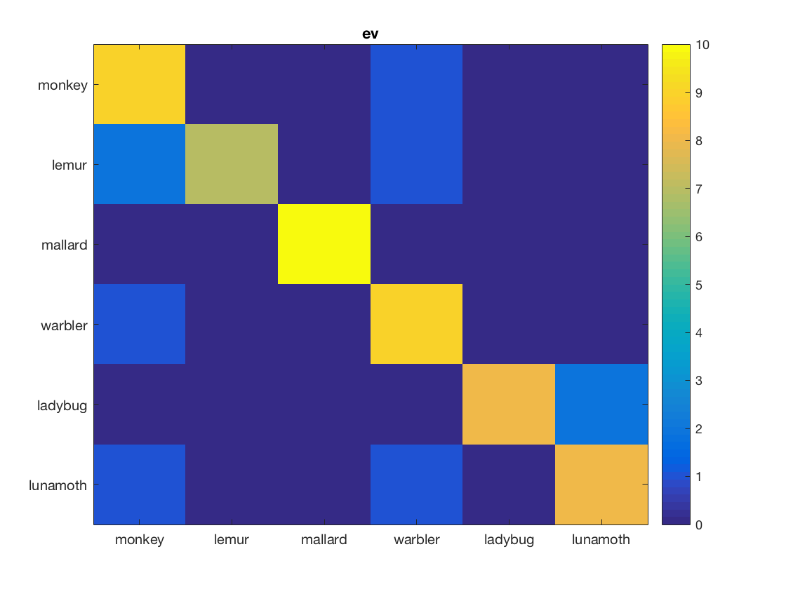
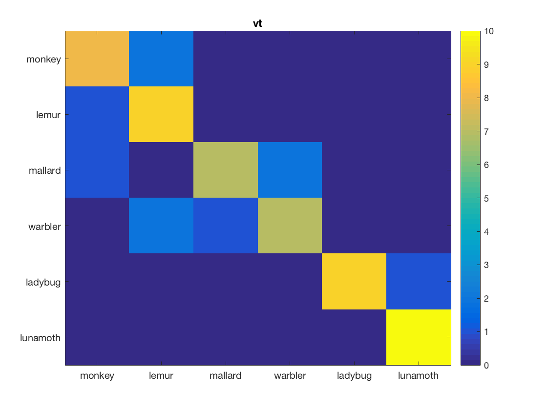
Part 4: (advanced) use cosmo_searchlight to get confusion matrices
% This exercise is like part 2 (classifation), but now
% classification confusions are computed and visualized
%
% set arguments for the measure, ensuring that the predictions (instead
% of classification accuracies) are returned
measure = @cosmo_crossvalidation_measure;
measure_args = struct();
measure_args.partitions = cosmo_nfold_partitioner(ds);
measure_args.classifier = @cosmo_classify_lda;
measure_args.output = 'predictions';

% apply searchlight using the dataset, neighborhood, measure, and measure
% arguments; store the result in 'ds_confusion'
% >@@>
ds_confusion = cosmo_searchlight(ds, nbrhood, measure, measure_args);
% <@@<

% show contents of ds_confusion
cosmo_disp(ds_confusion);

% convert to array form (nclasses x nclasses x nrois, with nclasses=6 and
% nrois=2) and assign the result to a variable 'mx_confusion'
% Hint: use cosmo_confusion_matrix and apply it to 'ds_confusion' directly
% >@@>
mx_confusion = cosmo_confusion_matrix(ds_confusion);
% <@@<

% visualize the confusion matrices

classes = {'monkey', 'lemur', 'mallard', 'warbler', 'ladybug', 'lunamoth'};
nmatrices = size(mx_confusion, 3);
for k = 1:nmatrices
    % >@@>
    figure();
    imagesc(mx_confusion(:, :, k), [0 10]);
    title(ds_confusion.fa.roi_names{k});
    set(gca, 'xtick', 1:numel(classes), 'xticklabel', classes);
    set(gca, 'ytick', 1:numel(classes), 'yticklabel', classes);
    colorbar();
    % <@@<
end
+00:00:00 [####################] -00:00:00
.a
  .some_attribute
    'useless'
.fa
  .roi_names
    { 'ev'  'vt' }
  .center_ids
    [ 1         2 ]
.samples
  [ 1         1
    1         2
    3         4
    :         :
    4         2
    6         5
    4         6 ]@60x2
.sa
  .targets
    [ 1
      2
      3
      :
      4
      5
      6 ]@60x1