RSA Visualize

Contents

Load data in EV and VT mask

load datasets cosmo_fmri_dataset

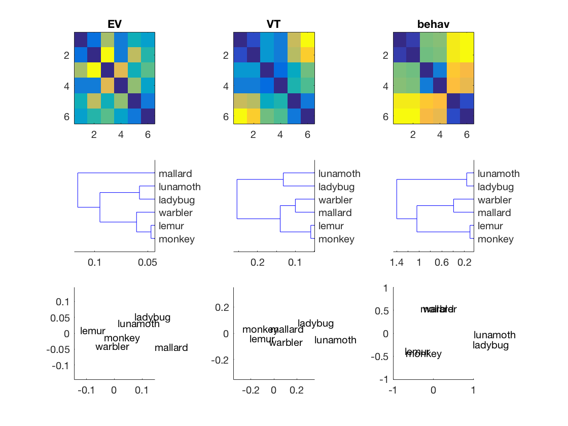
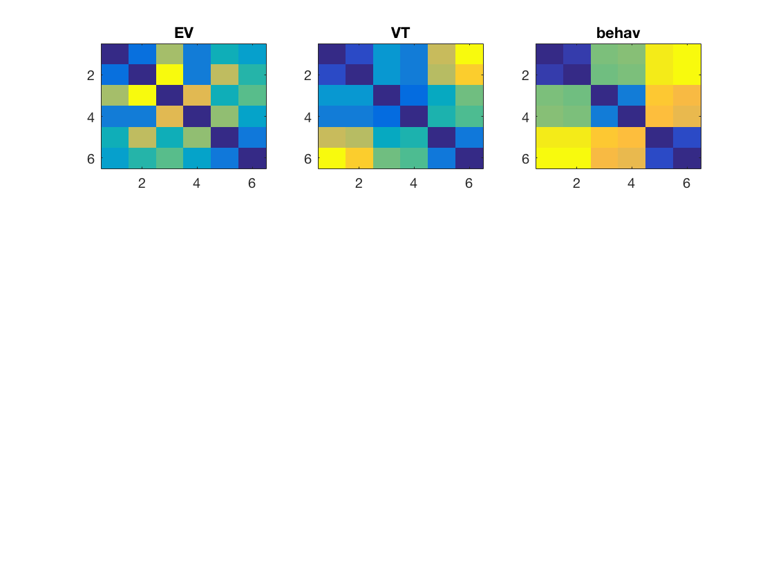
config = cosmo_config();
data_path = fullfile(config.tutorial_data_path, 'ak6', 's01');

data_fn = [data_path '/glm_T_stats_perrun.nii'];
targets = repmat(1:6, 1, 10)';
ev_ds = cosmo_fmri_dataset(data_fn, ...
                           'mask', [data_path '/ev_mask.nii'], ...
                           'targets', targets);

vt_ds = cosmo_fmri_dataset(data_fn, ...
                           'mask', [data_path '/vt_mask.nii'], ...
                           'targets', targets);

% compute average for each unique target, so that the datasets have 6
% samples each - one for each target
vt_ds = cosmo_fx(vt_ds, @(x)mean(x, 1), 'targets', 1);
ev_ds = cosmo_fx(ev_ds, @(x)mean(x, 1), 'targets', 1);

% remove constant features
vt_ds = cosmo_remove_useless_data(vt_ds);
ev_ds = cosmo_remove_useless_data(ev_ds);

% Use pdist (or cosmo_pdist) with 'correlation' distance to get DSMs
% in vector form. Assign the result to 'ev_dsm' and 'vt_dsm'
% >@@>
ev_dsm = pdist(ev_ds.samples, 'correlation');
vt_dsm = pdist(vt_ds.samples, 'correlation');
% <@@<

model_path = fullfile(config.tutorial_data_path, 'ak6', 'models');
load(fullfile(model_path, 'behav_sim.mat'));
behav_dsm = squareform(behav);

% Using matlab's subplot function place the heat maps for EV, VT
% and behaviour DSMs side by side in the top three positions of a 3 x 3
% subplot figure.
% (Hint: to convert DSMs in vector form to matrix form (and vice versa),
% using cosmo_squareform or squareform).

% >@@>
figure();

subplot(3, 3, 1);
imagesc(squareform(ev_dsm));
title('EV');

subplot(3, 3, 2);
imagesc(squareform(vt_dsm));
title('VT');

subplot(3, 3, 3);
imagesc(squareform(behav_dsm));
title('behav');
% <@@<

labels = {'monkey', 'lemur', 'mallard', 'warbler', 'ladybug', 'lunamoth'}';

Add the dendrograms for EV, LV and behav in the middle row of the

subplot figure (this requires matlab's stats toolbox)

if cosmo_check_external('@stats', false)
    % First, compute the linkage using Matlab's linkage for
    % 'ev_dsm', 'vt_dsm' and 'behav_dsm'. Assign the result
    % to 'ev_hclus', 'vt_hclus', and 'behav_hclus'

    % >@@>
    ev_hclus = linkage(ev_dsm);
    vt_hclus = linkage(vt_dsm);
    behav_hclus = linkage(behav_dsm);

    % <@@<

    subplot(3, 3, 4);
    % show dendrogram of 'ev_hclus'
    % As additional arguments to the dendrogram function, use:
    %      'labels',labels,'orientation','left'
    % >@@>
    dendrogram(ev_hclus, 'labels', labels, 'orientation', 'left');
    % <@@<

    % Using the same approach, show a dendrogram of 'vt_hclus'
    subplot(3, 3, 5);
    % >@@>
    dendrogram(vt_hclus, 'labels', labels, 'orientation', 'left');
    % <@@<

    % Using the same approach, show a dendrogram of 'behav_hclus'
    subplot(3, 3, 6);
    % >@@>
    dendrogram(behav_hclus, 'labels', labels, 'orientation', 'left');
    % <@@<
else
    fprintf('stats toolbox not present; cannot show dendrograms\n');
end

Show the MDS (multi-dimensional scaling) plots in the bottom row

% Show early visual cortex model similarity
subplot(3, 3, 7);

% get two-dimensional projection of 'ev_dsm' dissimilarity using cmdscale;
% assign the result to a variable 'xy_ev'
% >@@>
xy_ev = cmdscale(squareform(ev_dsm));
% <@@<

% plot the labels using the xy_ev labels
text(xy_ev(:, 1), xy_ev(:, 2), labels);

% adjust range of x and y axes
mx = max(abs(xy_ev(:)));
xlim([-mx mx]);
ylim([-mx mx]);

% Show VT similarity

% using cmdscale, store two-dimensional projection of 'vt_dsm' and
% 'behav_dsm' in 'xy_vt' and 'xy_behav'
% >@@>
xy_vt = cmdscale(squareform(vt_dsm));
xy_behav = cmdscale(squareform(behav_dsm));
% <@@<

subplot(3, 3, 8);
text(xy_vt(:, 1), xy_vt(:, 2), labels);
mx = max(abs(xy_vt(:)));
xlim([-mx mx]);
ylim([-mx mx]);

subplot(3, 3, 9);
text(xy_behav(:, 1), xy_behav(:, 2), labels);
mx = max(abs(xy_behav(:)));
xlim([-mx mx]);
ylim([-mx mx]);

Published with MATLAB® R2024a