Spherical searchlight
this example implements a spherical searchlight using cosmo_spherical_neighborhood and performs crossvalidation with a nearest neigh classifier
Note: for running searchlights it is recommended to use cosmo_searchlight and cosmo_spherical_neighborhood
- For CoSMoMVPA's copyright information and license terms, #
- see the COPYING file distributed with CoSMoMVPA. #
Contents
Set up parameters
config = cosmo_config();
data_path = fullfile(config.tutorial_data_path, 'ak6', 's01');
output_path = fullfile(config.output_data_path);

fn = fullfile(data_path, 'glm_T_stats_perrun.nii');
maskfn = fullfile(data_path, 'brain_mask.nii');
radius = 3;
targets = repmat(1:6, 1, 10);
chunks = floor(((1:60) - 1) / 6) + 1;
classifier = @cosmo_classify_nn;
classifier_opt = struct();
load data and set sample attributes
ds = cosmo_fmri_dataset(fn, 'mask', maskfn, ...
                        'targets', targets, ...
                        'chunks', chunks);

fprintf('Input dataset:\n');
cosmo_disp(ds);
Input dataset:
.a
  .vol
    .mat
      [ -3         0         0       121
         0         3         0      -114
         0         0         3     -11.1
         0         0         0         1 ]
    .xform
      'scanner_anat'
    .dim
      [ 80        80        43 ]
  .fdim
    .labels
      { 'i'
        'j'
        'k' }
    .values
      { [ 1         2         3  ...  78        79        80 ]@1x80
        [ 1         2         3  ...  78        79        80 ]@1x80
        [ 1         2         3  ...  41        42        43 ]@1x43 }
.sa
  .targets
    [ 1
      2
      3
      :
      4
      5
      6 ]@60x1
  .chunks
    [  1
       1
       1
       :
      10
      10
      10 ]@60x1
.samples
  [  0.933  0.000495       2.1  ...   0.681     0.626     0.421
    -0.772     0.117      1.73  ...   0.723     0.892       1.7
     0.621      1.52     -0.25  ...  -0.341    -0.832    -0.546
       :        :         :             :         :         :
     -2.37     -1.92    -0.879  ...   0.784      0.67     0.522
    -0.261     0.351   -0.0767  ...    2.81      2.27    -0.947
     -1.29    -0.964    -0.966  ...   0.827     0.833     0.991 ]@60x43822
.fa
  .i
    [ 35        36        44  ...  46        47        47 ]@1x43822
  .j
    [ 17        17        17  ...  35        35        36 ]@1x43822
  .k
    [ 1         1         1  ...  39        39        39 ]@1x43822
define centers of searchlight
nfeatures = size(ds.samples, 2);
center_ids = 1:nfeatures;
use voxel selection function
nbrhood = cosmo_spherical_neighborhood(ds, 'radius', radius);
center2neighbors = nbrhood.neighbors;
ncenters = numel(center2neighbors); % should be equal to 'nfeatures'
+00:00:00 [####################] -00:00:00 mean size 111.5
set up cross validation
(here we use cosmo_oddeven_partitioner; cosmo_nfold_partitioner would be another possibility, with the advantage of using a larger training set, but the disadvantage that it takes longer to run)
partitions = cosmo_oddeven_partitioner(ds);
Allocate space for output
ncenters = numel(center_ids);
accs = zeros(1, ncenters);
Run the searchlight
go over all features: in each iteration, slice the dataset to get the desired features using center2neighbors, then use cosmo_crossvalidate to get classification accuracies (it's its second output argument), and store the classiifcation accuracies.
Note: it is generally easier (and faster) to use cosmo_searchlight and cosmo_crossvalidation_measure; this example here is for illustrative purposes mainly
% use cosmo_show_progress to show a pretty progress bar
prev_msg = '';
clock_start = clock();
show_progress_every = 1000;
for k = 1:ncenters
    % >@@>
    center_id = center_ids(k);
    sphere_feature_ids = center2neighbors{center_id};

    sphere_ds = cosmo_slice(ds, sphere_feature_ids, 2);

    % run cross validation
    [pred_cv, acc] = cosmo_crossvalidate(sphere_ds, classifier, ...
                                         partitions, classifier_opt);

    % for now, just store the accuracy (not the predictions)
    accs(center_id) = acc;

    % <@@<

    % show progress every 1000 steps, and at the beginning and end.
    if k == 1 || mod(k, show_progress_every) == 0 || k == nfeatures
        mean_so_far = mean(accs(1:k));
        msg = sprintf('accuracy %.3f (%d features visited)', mean_so_far, k);
        prev_msg = cosmo_show_progress(clock_start, k / ncenters, msg, prev_msg);
    end
end
+00:00:41 [####################] -00:00:00 accuracy 0.202 (43822 features visited)
store the output
this uses the neighborhood from spherical voxel selection, after removing the fields neighbors and origin
res_map = nbrhood;
res_map = rmfield(res_map, {'neighbors', 'origin'});
res_map.samples = accs;
res_map.sa = struct();

% little sanity check
cosmo_check_dataset(ds);

fprintf('Output dataset:\n');
cosmo_disp(res_map);

output_fn = fullfile(output_path, 'spherical_neighborhood_searchlight.nii');
cosmo_map2fmri(res_map, output_fn);
fprintf('Output written to %s\n', output_fn);
Output dataset:
.a
  .vol
    .mat
      [ -3         0         0       121
         0         3         0      -114
         0         0         3     -11.1
         0         0         0         1 ]
    .xform
      'scanner_anat'
    .dim
      [ 80        80        43 ]
  .fdim
    .labels
      { 'i'
        'j'
        'k' }
    .values
      { [ 1         2         3  ...  78        79        80 ]@1x80
        [ 1         2         3  ...  78        79        80 ]@1x80
        [ 1         2         3  ...  41        42        43 ]@1x43 }
.fa
  .nvoxels
    [ 42        46        45  ...  41        41        38 ]@1x43822
  .radius
    [ 3         3         3  ...  3         3         3 ]@1x43822
  .center_ids
    [ 1         2         3  ...  4.38e+04  4.38e+04  4.38e+04 ]@1x43822
  .i
    [ 35        36        44  ...  46        47        47 ]@1x43822
  .j
    [ 17        17        17  ...  35        35        36 ]@1x43822
  .k
    [ 1         1         1  ...  39        39        39 ]@1x43822
.samples
  [ 0.2    0.0833      0.35  ...  0.267     0.183     0.117 ]@1x43822
.sa
  struct (empty)
Output written to /Volumes/andor/tmp/CoSMoMVPA_output/spherical_neighborhood_searchlight.nii
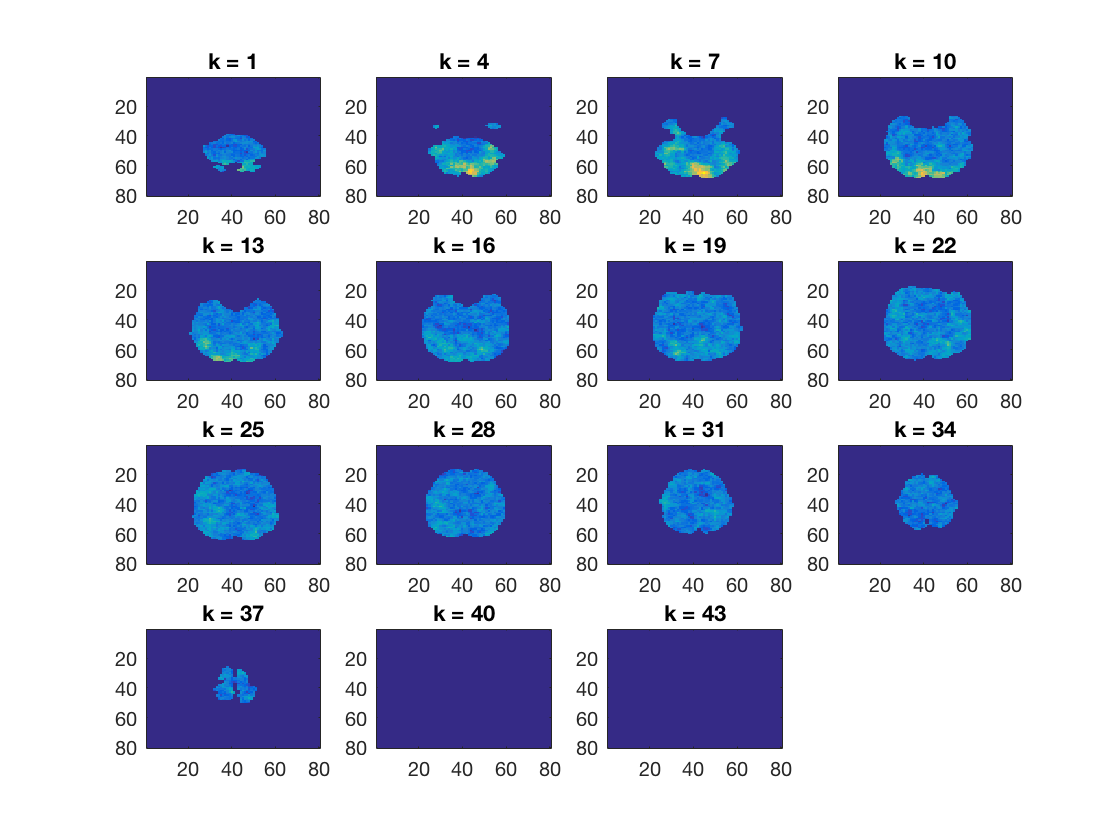
Plot a few slices
cosmo_plot_slices(res_map);
