Classification analysis

Reading material

• [CS03]: First use of a classifier on fMRI data.

• [MBK09]: Classification introduction and overview.

Background

This exercise shows a more advanced MVPA topic, the use of a classifier (first reported in [CS03]). Using a classifier involves two steps:

• training: a set of samples (the patterns) with associated .sa.targets (conditions) together are called the training set. The training set is used so that the classifiers learns which patterns are associated with each condition.

  • (side note: learning associations between patterns and conditions can be done in many ways. Popular approaches are Naive Bayes, Linear Discriminant Analysis, and Support Vector Machines (Nearest Neighbor classification is another approach, but less useful for fMRI data). They make different assumptions about the distribution of the patterns and what is the best way to separate patterns from different conditions). When in doubt which classifier to use, one recommendation is to use either LDA or SVM. The former seems less popular in the literature, but is typically faster and has fewer free parameters (thus potentially reducing a researcher’s degrees of freedom).

• testing: predict the conditions (.sa.targets) for another set of samples (the test set), to see how well the classifier can generalize to a new set of data.

Classification performance can be assessed by considering how many predictions for the set set were correct.

• No peeking is allowed.

  • During the testing step, the classifier is not allowed to peek at the conditions. Otherwise it could just use those conditions and classification would always be perfect.

• No double dipping.

  • The training and test set must be independent. In CoSMoMVPA, independence can be indicated by the .sa.chunks attribute. In fMRI data, usually one takes one chunk value for each data acquisition run. If the data were not independent, then the classifier could overtrain on the training data but unable to generalize to new, independent data.

• Multiple samples in each class are required (almost always).

  Unlike the cosmo correlation measure, a classifier usually requires that the training set has multiple samples of each class. It can use this information to assess, for example, variability of responses in each feature. This makes a classifier potentially more sensitive than a standard split-half analysis (Split-half correlation-based MVPA with group analysis).

• How to assess classification performance?

  • A very stupid classifier, one that would not even look at the data, could, for example

    • either predict all samples in the test set to belong to the same classes (e.g. the first one), or

    • predict a random class for each sample in the test set.

  • In this case, if there are C classes (unique targets), which each class occuring equally often, then each sample in the test set has a chance of being predicted correctly of 1/C (the chance level). For example, with four classes, each sample would be predicted correctly with a chance of 1/4, or 25%.

  • If a set of patterns an a region of interest actually contains information about the conditions (i.e, is an informative region), and the classifier is able to use this information, then classification performance would be above chance level.

  • If a group of participants all show classification accuracy above chance consistently, one can claim that the region of interest contains information about the the conditions. A simple one-sample t-test against chance level can be used to obtain a statistic and associated p-value.

A single classification step can be visualized as follows (more advanced cross-validation is part of another exercise):

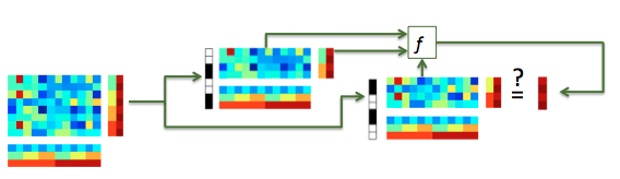
Illustration of (single-fold) classification. A dataset (left) is split in a train dataset (top dataset) and a test set (bottom dataset), which must have no chunks in common. For training, a classifier (indicated by f) takes .samples and .sa.targets from the train dataset (horizontal arrow into f) and predicts, for the .samples in the test set (vertical arrow into f), the targets of the test set (U-turn arrow). Classification accuracy can be assessed by computing how many samples in the test set were predicted correctly.

Single subject, single fold split-half classification

Before starting this exercise, please make sure you have read about:

• Classifier

For this exercise, load a dataset using subject s01’s T-statistics for every run (‘glm_T_stats_perrun.nii’) and the VT mask.

Slice (using cosmo slice) the dataset twice to get odd and even runs.

Part 1:

• Slice the odd and even runs again so that there are only two categories: warblers and mallards.

• Train and test a LDA (linear discriminant analyses; cosmo classify lda) classifier, training on the even-runs data and testing on the odds.

• Compute classification accuracy

• Repeat the previous two steps using cosmo classify naive bayes

Advanced exercises:

• What is the accuracy for monkey versus ladybug? Monkey versus lemur?

• What if you use the EV mask?

Part 2:

• Use the data from all six categories to train on even runs and test on odd runs, and compute the classification accuracy.

• As the previous step, but now test on odd runs and test on even runs.

Part 3:

• Using the predictions and the true labels (targets), show a confusion matrix that counts how often a sample with targets==i was predicted to have label j (for i, j both in the range 1:6). How can you interpret this matrix?

Template: run classify lda skl

Check your answers here: run classify lda / Matlab output: run_classify_lda